Congestion control in TCP

Congestion control is use to utilise the network with the following goals in mind:

• Efficiency: We should try to have high utilisation of the network at all times.
• Fairness: Each user should have a fair share of the network.
• Low delay: We should not overwhelm the switches and routers buffers causing a large delay within the network.
• Fast convergence: We want to get to a stable point that achieves all the above quickly.

There are two approaches when it comes to congestion control.

• Network assisted: You rely on the network to provide some signal about how congested it is. This could be done via:
  • ICMP source quench.
• End-to-end congestion control: Hosts need to infer congestion from the traffic they receive. This can use different signal such as:
  • Packet delay based on acknowledgement times.
  • Packet loss using the acknowledgement sequence numbers.
  • Major network delay based on the time out window.

TCP uses the end-to-end approach. It mainly uses packet loss to detect congestion as packet delay can have quite a bit of noise in the system. It uses major network delay to reset itself.

TCP uses ACK messages as a probes and adopts a probe-and-adapt approach to adjusting the window size (number of unacknowledged packets) for congestion control.

Additive increase Multiplicative Decrease (AIMD)

Additive increase Multiplicative Decrease (AIMD)

This is a method of probe-and-adjust that some TCP implementations use.

• Every RTT it wants to increase the window size by 1.
• If there is congestion on the network it halves the window size.

As the window size is really in bytes rather than packets and we would like incremental progress rather than waiting for a full RTT. We increment the window size using the maximum segment size (MSS) proportionally to the current CongestionWindow size on every acknowledged packet using the formula:

Link to original

TCP Reno

TCP Reno

This is the classical Congestion control in TCP. It starts the window size to be 1 packets big. It uses AIMD with two different signals.

• If a message is waited on 3 times, it halves the congestion window in AIMD.
• If it reaches a timeout window (i.e. no message is received for a given length of time). It resets the congestion window back to 1.

This however is quite slow to start. Therefore Reno implements “slow start” doubling up to some threshold. This means that while the congestion window is below the that threshold every RTT it doubles the congestion window. Once it passes this threshold or it drops a packet it switchest back to AIMD The “slow start” also takes place if we have a timeout. In this case the threshold is set to be the congestion window before the timeout.

Link to original

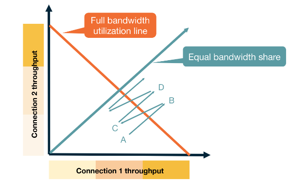
Fairness

This achieves fairness through AIMD. As the punishment for dropping a packet is exponential vs an increase which is linear. If you are using more of the network your probability of dropping a packet is higher and equally that punishment is larger. Whilst you are not dropping packets your increase is the same as every other network participant.

This exponential vs linear dynamic allows for fast convergence to an equilibrium.

Fairness between connections not applications

If one application has multiple open connections each connection will reach a fair state but an application with many connections will have an unfair share of the network.

TCP CUBIC

TCP CUBIC

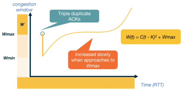
In networks with large bandwidth or a long delay TCP Reno yields low network utilisation. TCP CUBIC is the more efficient implementation used within the linux kernal. CUBIC still uses a reset for a timeout and halves when it gets a triple unacknowledged message. Though this implementation uses two different features to TCP Reno:

• A cubic polynomial increase function.
• Increase is based off the time since the last packet loss instead increasing when it gets an ACK packet.

Let be the window size, and lets say we are given two constants and . Suppose we get a packet loss when is at and let be the time since that event. First set then we set our window size to be

Link to original

Throughput

Assuming we have a probability of of dropping a message - we can model what our expected throughput is for TCP Reno. For this model we assume the network delivers packets then drops one. This provides the following saw-tooth diagram.

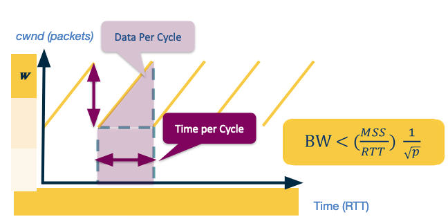
Assume the max window size is , then as the number of packets is increasing linearly we have the width and height of the saw is . Therefore the total packets sent is

Which using our assumption means that

Therefore we can compute the bandwidth of this connection.

We set to be a constant as we can study this in practice rather than just in theory. In practice we see that is regularly less than 1, so we say

Data Centres

In Data Centres we see a lot of developments in TCP implementations for congestion control. There are two main reasons for this:

• Data centres make lots of delay sensitive short messages that normal TCP wouldn’t handle well.
• Data centres are owned by a single entity so they can deploy different algorithms much easier.