Week 6 - Graph algorithms - strongly connected components

DFS - not the sofa seller!

Recall the definition of Depth-first search (DFS) in the note. We used it there to find the connected components of a graph.

DFS to find connected components in an undirected graph

DFS to find connected components in an undirected graph

To solve the following problem.

Statement

Find connected components in an undirected graph

Given a graph how can we find a mapping from it’s vertices to the connected components of .

Link to original

We can use the following DFS algorithm.

DFS(G)
  input: G = (V,E) in adjacency list representation
  output: Vertices labelled by connected components
    connected_component = 0
    for all v in V, set visited(v) = False
    for all v in V
      if not visited(v) then
        connected_component++
        explore(v)
    return connected_component_number (defined in explore)

Explore(z)
  input: vertex z
  output: side effect, it defines the connected component_number on some vertices and marks them as visited.
    connected_component_number(z) = connected_component
    visited(z) = True
    for all (z, w) in E
      if not visited(w)
        Explore(w)

As we run through every vertex once and then every edge twice we have .

Link to original

Find paths in undirected graph via DFS

First for undirected graphs we just keep track of the previous vertex and find a spanning sub-forest for the graph. We can use this to find paths between vertices by going back to the root vertices of the trees.

DFS(G)
  input: G = (V,E) in adjacency list representation
  output: Vertices labelled by connected components
    connected_component = 0
    for all v in V, set visited(v) = False, previous(v) = Null
    for all v in V
      if not visited(v) then
        connected_component++
        explore(v)
    return previous

Explore(z)
  input: vertex z
    connected_component_number(z) = connected_component
    visited(z) = True
    for all (z, w) in E
      if not visited(w)
        previous(w) = z
        Explore(w)

Find paths in undirected graph via DFS

To do this we are going to use a DFS algorithm like above but we are going to track pre/postorder numbers.

DFS(G)
  input: G = (V,E) in adjacency list representation
  output: Vertices labelled by connected components
    clock = 1
    for all v in V, set visited(v) = False
    for all v in V
      if not visited(v) then
        explore(v)
  return post (defined in Explore)

Explore(z)
  input: vertex z
    pre(z) = clock, clock ++
    visited(z) = True
    for all (z, w) in E
      if not visited(w)
        Explore(w)
	post(z) = clock, clock++

Example

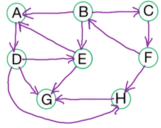
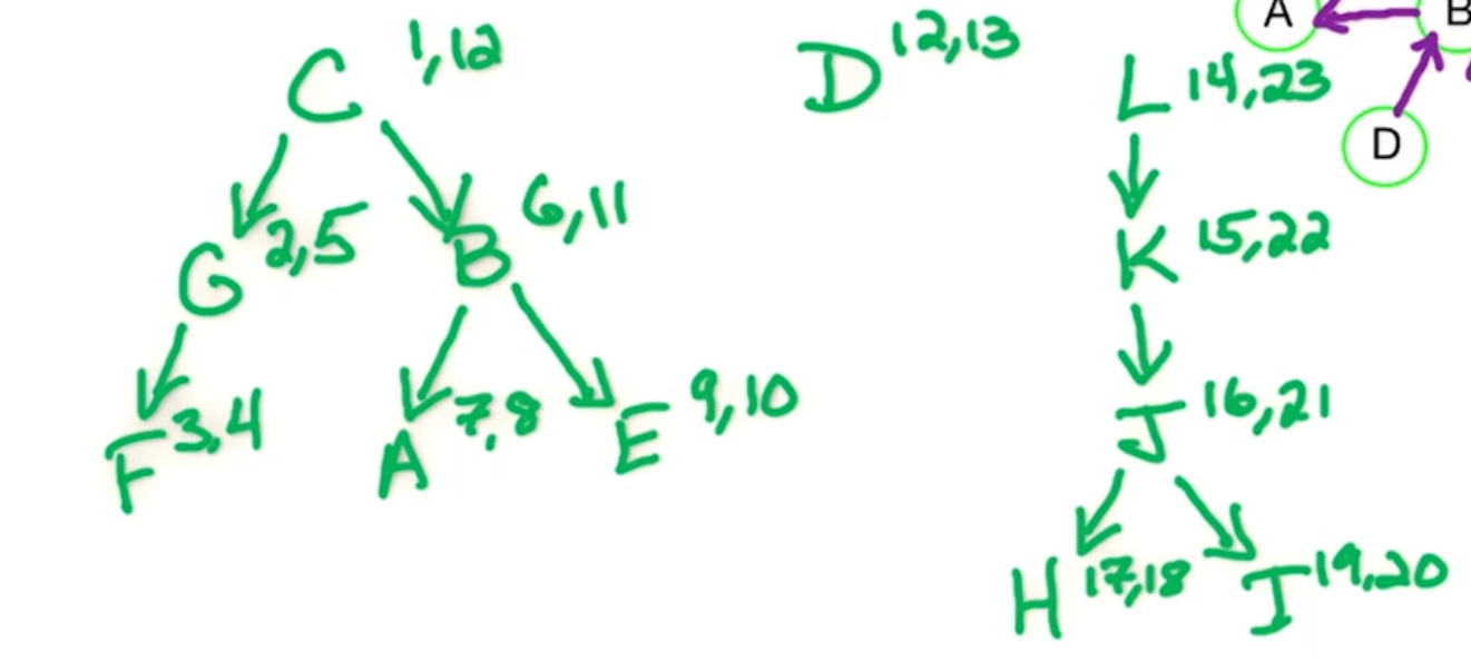
Suppose we have the following graph and let be the root node. Suppose we explore edges alphabetically and lets run the algorithm above on it.

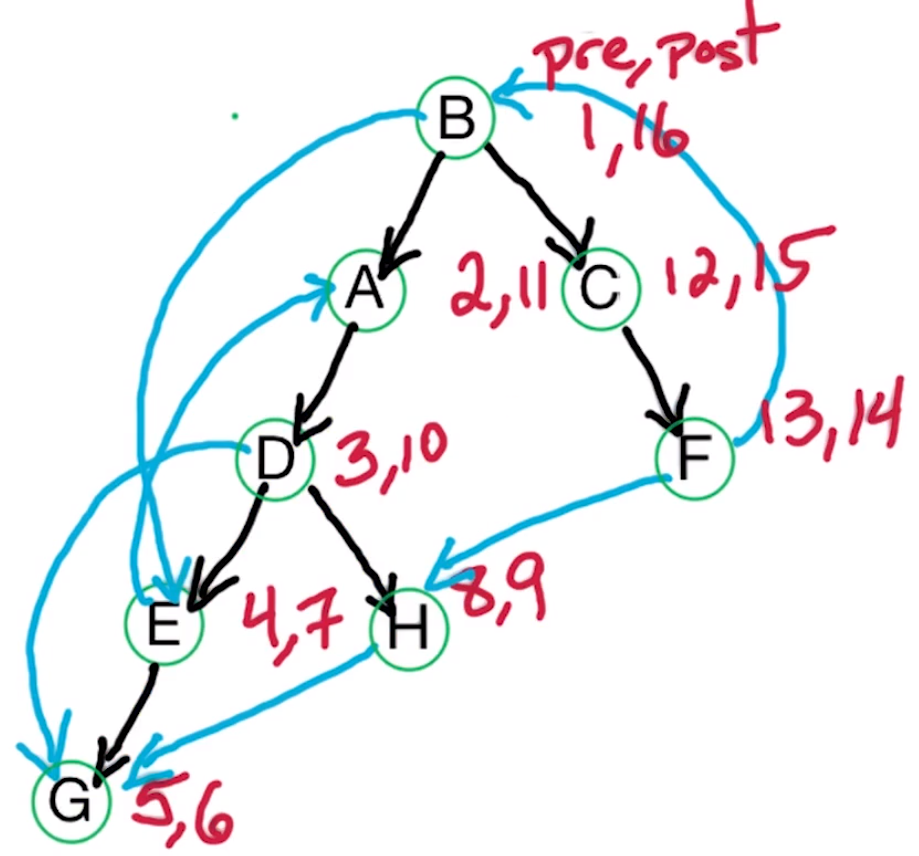
As we are using DFS we explore far first and then slowly come back. Which gives us the following DFS tree with the pre/post numbers.

Letter	Pre	Post
A	2	11
B	1	16
C	12	15
D	3	10
E	4	7
F	13	15
G	5	6
H	8	9

Lets try and classify the edges in this graph

• Tree edges
  • First explored edges (black) that form a spanning subgraph.
  • Examples: ,
• Back edges
  • Edges going from a node further out from the root (in the black edges) to a node closer to it but still in the same branch.
  • Examples ,
• Forward edges
  • Edges that go further down the tree.
  • Examples: ,
• Cross edges
  • Edges that go from one branch to another.
  • Examples: ,

Note here there the only type of edges to have are back edges.

Cycles in a graph via the DFS tree

Lemma

A directed graph has a cycle if and only if its DFS tree has a back edge.

Proof

Suppose we have a graph and some run of a DFS algorithm that forms DFS tree .

Suppose it has some cycle where and . Then some vertex must have been discovered first by .

All other vertices must be below and contained in its branch. Therefore is contained in its branch with edge giving the desired back edge.

Suppose we have some back edge . By the definition of back edge but and are in the same branch in .

Therefore there are edges connecting to in making a cycle.

Link to original

Topological sorting

Topological sorting (DAG)

Topological sorting

Suppose we have a DAG a topological sorting on is a linear ordering of such that for all edges we have .

Link to original

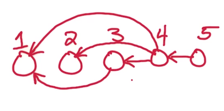
Suppose we have a DAG from the lemma above we can run a DFS algorithm starting at the root of and the post ordering will provide a topological sorting of the vertices of .

Vertices in a DAG

We can classify special vertices in a DAG

• Source vertices: These have no incoming edges
• Sink vertices: no outgoing edges

Given a linear ordering we know the minimal vertex is a source and the maximal vertex is a sink. This gives us another algorithm to find a topologically sorting:

1. Find a sink vertex, label it and then delete it.
2. Repeat (1) until the graph is empty

Strongly connected components

Recall the definitions

Strongly connected (directed graphs)

Strongly connected

Let be a directed graph. We say two vertices are strongly connected if there exists paths to and to .

Link to original

Strongly connected components (directed graphs)

Strongly connected components

Let be a directed graph. We say is a strongly connected component if all vertices are strongly connected and is maximal with this property.

Link to original

Then we can define the strongly connected component graph

Strongly connected component graph (directed graph)

Strongly connected component graph

Let be a directed graph. Suppose has strongly connected components . We can define the strongly connected component graph as a directed graph with vertices and edges

Link to original

Which we can show is a DAG.

The strongly connected component graph is a DAG

Lemma

The strongly connected component graph is a DAG.

Proof

Let be directed graph.

Suppose two strongly connected components and in had paths connecting to and connecting to .

As and are strongly connected components we know there are paths , connecting to and vice versa as well as to .

However, connects to and connects to giving is not maximal. Therefore no such set of paths and exist.

Therefore no cycle can exist in the strongly connected component graph either.

Link to original

Strongly connected component algorithm

The idea of the algorithm is the following:

• Find a sink strongly connected component,
• Remove it,
• Repeat!

We use sinks as if we start a DFS algorithm in a sink strongly connected component we only discover vertices in that strongly connected component.

This is not true for source strongly connected components, here we discover everything.

Finding a vertex in a sink SCC

We have the following two statements in a DAG:

• The vertex with the lowest postorder number is a sink.
• Then vertex with the highest postorder number is a source.

We would hope for the analogous statements in a general directed graph:

• The vertex with the lowest post order number is in a sink strongly connected component
• The vertex with the highest post order number is in a source strongly connected component

The first statement is false consider the following counter example.

Transclude of sink_counter_example

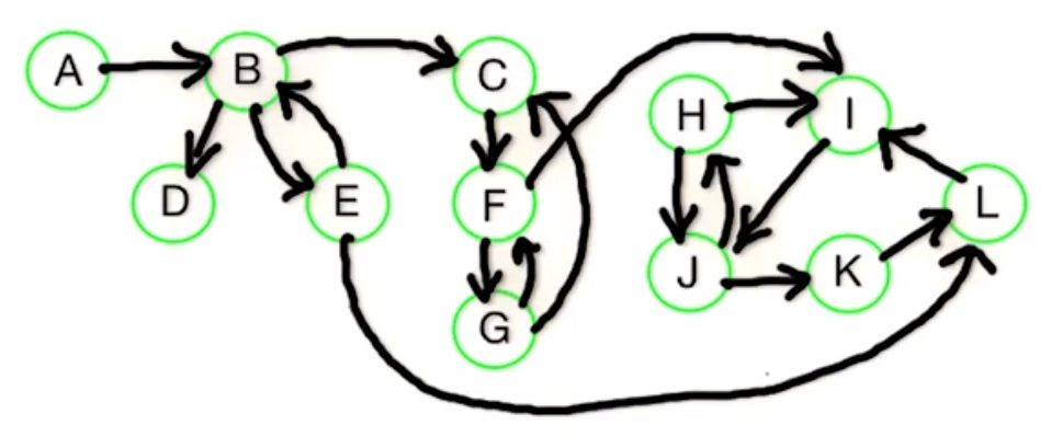
If we run a DFS algorithm starting at using an alphabetical ordering on the vertices then has the lowest post order number but is in the source strongly connected component.

A vertex with the highest post order number lies in a source SCC

Lemma

Suppose we have a directed graph and be the result of running the DFS to find connected components in an undirected graph algorithm. Then the vertex with the largest post order number lies in a source strongly connected component in the strongly connected component graph.

Proof

Let be the strongly connected component with the vertex of highest value.

Suppose some other strongly connected component were to have an edge connecting to in the strongly connected component graph.

From the Lemma has a vertex with higher post order than all vertices in . This is a contradiction as contains the vertex with highest post order.

Link to original

Suppose we a directed graph define the reverse directed graph . Now observe

The strongly connected components are the same in a directed graph and its reverse

Lemma

Let be a directed graph and be its reverse. Both and have the same strongly connected components.

Proof

For any two vertices who are strongly connected in we need a path connecting to and path connecting to .

The reverse of the path connected to in and connects to in .

Therefore if two vertices are strongly connected in they are strongly connected in .

As this also gives us that if two vertices are strongly connected in they are strongly connected in .

Thus by the definition of strongly connected components they must be identical in and .

Link to original

Moverover we have.

Taking the reverse respects going to the strongly connected component graph

Lemma

Let be a directed graph and be its reverse. Then if is strongly connected component graph of then the reverse of is equal the strongly connected component graph of called . I.e. .

Proof

As the strongly connected components are the same in a directed graph and its reverse we know and have the same vertex set.

The edge set for is therefore the edge set for is Which by the definition of reverse could be rephrased as This is exactly the definition of the edge set for giving the required statement.

Link to original

Therefore if we can find a source vertex in then we have found a sink vertex in . This is exactly what our algorithm will depend on.

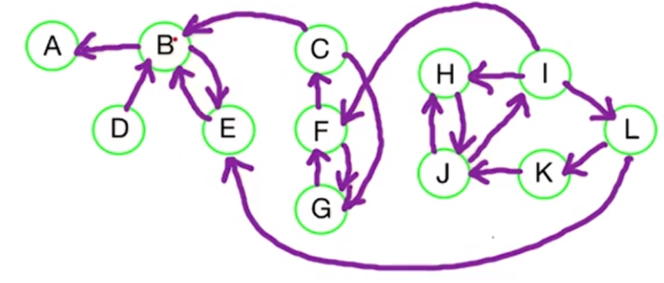
Algorithm for finding the strongly connected components

SCC(G):
	Input: directed graph G = (V,E) in adjacency list
	Output: labeling of V by strongly connected component
		1. Construct G^R
		2. Run DFS on G^R
		3. Order V by decreasing post order number.
		4. Run directed DFS on G using the vertex ordering from before and
		   label the connected components we reach.

Additional property

In addition to labelling the connected components the order we have labelled them is in reverse topological ordering. This is because we always start at the next sink vertex after we have labelled a component.

This takes as we do two runs of a DFS algorithm.

Example

Suppose we want to find the strongly connected components of the graph below.

First we look at and run the DFS to find path in an undirected graph algorithm.

This gives us - in this example we started at and did a fairly random vertex ordering.

Letter	Pre	Post
A	7	8
B	6	11
C	1	12
D	12	13
E	9	10
F	3	4
G	2	5
H	17	18
I	19	20
J	16	21
K	15	22
L	14	23

Then we order the vertices by reverse post order.

Letter	L	K	J	I	H	D	C	B	E	A	G	F
Post	23	22	21	20	18	13	12	11	10	8	5	4

Now run a connected components DFS using the vertex ordering above.

Letter	L	K	J	I	H	D	C	B	E	A	G	F
Post	23	22	21	20	18	13	12	11	10	8	5	4
CC	1	1	1	1	1	2	3	4	4	5	3	3

Notice also that the strongly connected component graph is the following.

Giving that our ordering is exactly a reverse topological sorting.