If you have access to the Kurose-Ross book and the Peterson book, you can find the list of chapters discussed in this lecture. As mentioned in the course schedule, purchasing the books is not required.
Kurose-Ross (6e)
4.5.1:The Link-State (LS) Routing Algorithm
4.5.2: The Distance- Vector (DV) Routing Algorithm
4.6.1: Intra-AS Routing in the Internet: RIP
4.6.2: Intra-AS Routing in the Internet: OSPF
Kurose-Ross (7e)
5.2.1The Link-State (LS) Routing Algorithm
5.2.2: The Distance- Vector (DV) Routing Algorithm
5.3: Intra-AS Routing in the Internet: OSPF
Kurose-Ross (8e)
5.2.1: The Link-State (LS) Routing Algorithm
5.2.2: The Distance- Vector (DV) Routing Algorithm
The process of routing is getting a packet the network associated to its IP address. To do this all routers store a routing table which maps the tuple of an IP address and a network mask to either a interface or a IP address.
There are 3 ways a router can populate its routing table
Directly connected: This is for networks directly connected to the router. It adds an entry for that networks and the interface of the router it is connected to.
Static route: This is a route that has been manually configured on a router. Instead of an interface it will have an IP address to forward that packet on to.
Dynamic routing: This is the same in structure to the static rout but instead of being manually added this gets populated by routers sharing known addresses with one another.
This table might grow very large but routers use route summarization to keep the tables shorter.
Once a router has been configured when it receives a packet it looks at its layer 3 header containing the destination IP address. It compares that again the known address, using the network mask and finds the most precise match (matching on the longest network mask) then forwards it to that interface or IP address.
Here are two main algorithms, these use two different approaches to how route packets.
Link-state routing algorithms
Link-state routing algorithms
Link-state algorithms are used for intradomain routing. These use knowledge of the whole network - including topology and weights - to perform Dijkstra’s algorithm on the network to find the shortest path to every node. This gives us where to route packets to. The computational complexity of this is where is the size of the network.
Distance vector routing is a distributed routing algorithm. It uses the Bellman-Ford algorithm but in a distributed manner.
For this was assume all routers know the routers they are directly connected to - within a network they have an interface to. They also know the network cost of communicating with their neighbours.
Each router maintains a table with all routers within their AS to each they associate, that routers best guess at the distance to the router, and which neighbour router they need to send any packets to to achieve that best guess.
Then all the routers broadcast this information to its neighbours and use their neighbours broadcasts to update their own tables. They update their tables using the Bellman-Ford equation.
This has a Count to infinity problem where if the distance of a connection is increased dramatically or it is removed then two neighbours might keep thinking the fastest rout is via one another as there distances and dependent on that edge not being changed. This causes a very slow convergence to the real path. We can improve the algorithm to account for this however this algorithm will still be vulnerable to this with large graphs.
This has the pseudocode as below.
Pseudocode
Let us have an AS which is represented by an undirected graph where each of are routers and an edge indicates they have a common network that belongs to their interfaces. Suppose this has a distance metric associated to it . Then we describe an algorithm for a particular vertex who has neighbours . This will build two maps - current best guess of the shortest distance and
-- InitalisationSet map D(v) = inf, S(y) = - for all v in V.Set D(x) = 0Set D(n) = d(x,n), S(n) = n for n in N_xSend D to all members of N_x.-- Recieve a messageSuppose we get D' from y in N_xFor every v in V where S(v) = y: # Can not use min here incase the distance has increased due # to network changes Set D(v) = d(x,y) + D'(v)For every v in V where S(v) /= y: Set D(v) = min(D(v), d(x,y) + D'(v)) Update S(v) = y if D(v) decreasedIf any value of D changes: # Handle to count to infinity problem For each n in N_x: Let D' be a copy of D For each v in V where S(v) = n: Set D'(v) = inf Send D' to n
This is a problem within the Distance vector routing algorithms caused by a change in the underlying graph or its distances. This causes very slow convergence to the correct intradomain distances as nodes all believe sending messages to one another using the old distances is the shortest path.
Example
Suppose we have an AS with 3 routers which are all connected to one another with initial distances and then we have the following shortest path tables.
D(r,c)
x
y
z
x
0
1
1
y
1
0
2
z
1
2
0
The suppose the edge breaks. If the Distance vector routing algorithms don’t take this problem into account then we get a slow escalation of distance.
Router requests its neighbour distances it updates and broadcasts this. Then updates its distances and broadcasts this. Then the problem goes on.
Avoidance
To get around this we track who we are planning on sending the update two to achieve the current minimum distance. If that is the same as the person we broadcast to then we set that distance to infinity. This method is called Poison reverse.
Whilst this solves the simple cases like above - it is easy to imagine chains for routers having this exact problem without being able to realise it.
This is one of the first protocols that implemented Distance vector routing algorithms. For the distance metric it just used the number of different routers it would have to go through.
The messages each router sends are the routing table with each subnet, the next router it would go through and the distance to that network in terms of “hops”. This table is refereed to as the RIP table. Later iterations of RIP use address aggregation.
To maintain connection with their neighbours they use a UDP message on port 520 if they don’t hear from neighbours every 180 seconds they will assume they are no longer available and change the RIP table then broadcast it to its neighbours.
This algorithms has challenges with updating routes and the time that takes to converge due to the count to infinity problem.
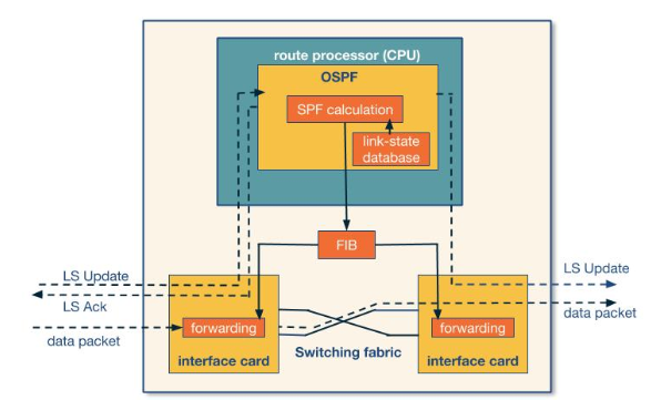
In OSPF a single router is selected as the backbone router this is where all AS externally facing routers connect to.
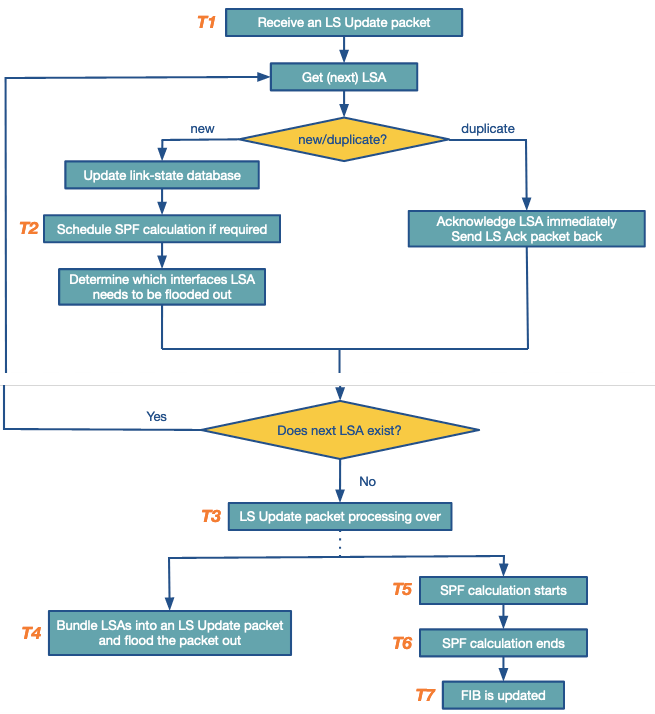
Routers withing the AS broadcast Link state advertisements (LSA) which include that routers neighbours. This is circulated to the whole network and is repeated at a set interval (normally 30 minutes). Then every router using itself as the root uses Dijkstra’s algorithm to find the shortest path between itself and every other subnet.
This can be summarised by the following flow chart.
Hot potato routing
Hot Potato Routing
This is the term used when deciding between two external egress routes to the Autonomous system (AS). Routes use he external egress that has the shortest intradomain routing distance.
The process of deciding the weights between routers can be complicated as small changes in weights can have a large impact to the traffic flow. There is a framework for this.
Measure: Observe how the network flow is happening at the moment. This involves looking at the current set of shortest paths and the capacity of each of the links.
Model: Predict how a change in weights would effect the these paths and capacities on the wires.
Control: Update the weights of the routers and go back to the first step to check your model was correct.