Week 11 - Linear Programming

In broad terms a linear programme is an optimisation problem of a linear function where there are linear bounds on the variables.

Max flow problem

We are given a directed graph with capacities and source and sink .

To define the linear programme make variables for each . These will represent the flow along these edges. Then we want to maximise the flow defined by the flow out of However, the edges must flow abiding by the capacity constraints As well as abide by the preservation of flow This defines our linear programme and the solution to this provides a solution to the max flow problem.

Linear programme general form

Linear programme

Linear programme

A linear programme has variables for where we are trying to either for some constants for . This is subject to linear constrains of the form for some constants with and .

Link to original

It helps to standardise this into the following form. Note the use of matrix notation here.

Linear programme standard form

Linear programme standard form

The standard form for a linear programme with variables and constraints is given by matrices , , and were we want to Some variants may use instead of in the objective function or use instead of in the constraints equation however this can easily be translated using the rules from the standard form lemma.

Link to original

We can convert all linear programmes into standard form using the following Lemma.

All linear programmes can be represented in standard form

Statement

Lemma

All linear programmes can be represented in standard form.

Proof

Suppose we have a Linear programme of generic form. We need to turn this into a standard form where:

• We are maximising an objective function,
• All constraints use the same inequality, and
• All variables are greater than zero.

If the objective function is this can be converted to a maximum by instead looking at Suppose we have an equality constraint this can be converted into two inequalities Suppose we have greater than or equal to inequality this can be converted into a less than inequality by multiplying through by negative one Lastly suppose we have a variable that can be negative. We can separated it into its positive and negative components where . We can then replace the use of by using the before substitution.

This transformation into a general form may increase the number of variables and number on constraints.

Link to original

Geometric view

From now on we just consider linear programmes in standard form.

We can consider the feasible such that and .

As there are variables we know , more over as we have that it lies in the positive region on .

Each row of defines a half space, so the feasible lie in the positive region of cut out by these half spaces.

2D-example

Suppose we have the linear programme with respect to and This region can be visualised as follows.

Transclude of 2d_feasible_region

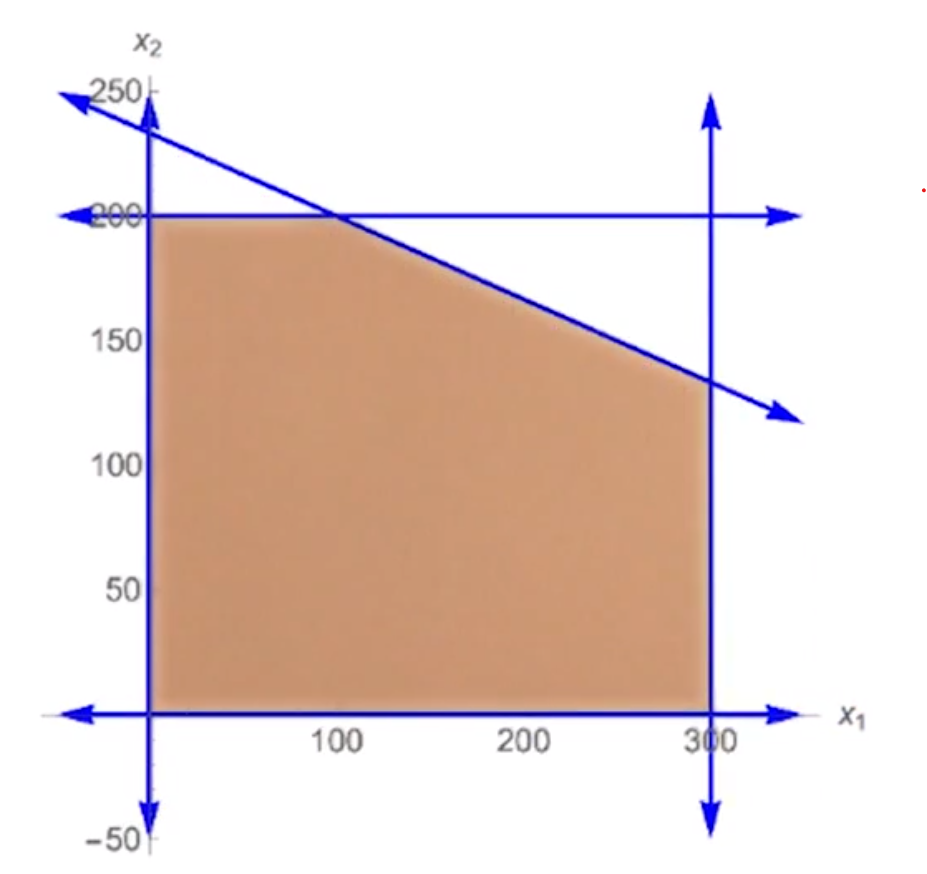
So the feasible region is cut out by half spaces in .

The vertices in this feasible space are ones that lie on a 0-dimensional intersection of the boundary of the half spaces. In the example above these would be

Linear programme solvers

When it comes to solving a linear programming problem.

Statement

Linear programme problem

Given a linear programme what is an that achieves an optimal solution if it exists.

Link to original

There are polynomial time algorithms like the ellipsoid method and interior-point method but in practice these can be slower than the much more widely used simplex method which can be exponential in its worst cases.

Simplex method

As vertices are extremal points with regards to the constraints we have that if the maximum of the objective function exists then it must be achieved on one of the vertices. Therefore the idea of the simplex algorithm is to start at a vertex then compare the objective function to all other vertices connecting to it.

So in short

1. Start at x = 0, if that is feasible.
2. Find all vertices adjacent to x along an edge.
3. compare the objective function of all vertices and
	1. If the current x is highest return that value.
	2. Switch x to be the highest of the objective functions found around x.
4. Go to step 2.

This only works if there is a point in the feasible region that achieves this maximum. Here we have 2 constraints:

• There is a point in the feasible region.
• That some point achieves a maximum - this happens when the region is bounded and has finite volume.

These are summarised by the two types of linear programme.

Infeasible linear programme

Infeasible linear programme

A linear programme is infeasible if there are no that satisfy its constraints.

Link to original

Unbounded linear programme

Unbounded linear programme

A Linear programme is unbounded if the value of the objective value can be arbitrarily large and so is not bounded above.

Link to original

Determining if a linear programme is infeasible

Suppose we have a linear programme in standard form which may or may not be a Infeasible linear programme. For any inequality and we can satisfy it by adding an arbitrarily small to the left hand side If we now that the original satisfied the inequality.

In summary from our original linear programme we can extend it to include an ‘th variable . We augment the constraints to include this variable on the left hand side. This is now a feasible linear programme.

Moreover, we can change the objective function of the linear programme to simply maximise and if that value is positive we have a feasible point in the original linear programme.

Checking if a linear programme is feasible

Checking if a linear programme is feasible

Suppose we are given a linear programme in standard form specified by , , and and we have a standard form linear programme solver .

Note we will include in the algorithm some transformation to guarantee the inputted linear programme is in standard form by breaking up the added variable into it’s positive and negative components. See getting a linear programme in standard form

feasibility_check(A, b):
	Input: The constraints to a linear programme in standard form.
	Output: If the linear programme is feasible.
1. Extend A with a column of 1's and another column of -1's at the end, making A' size m x (n+2).
2. Set objective function c = (0, 0, ..., 0, 1, -1) of length n+2.
3. Run linear_programme_solver(A', b, c).
4. If the value of the objective function is positive output it is feasible.
5. Otherwise say it is not.

Link to original

Aside: How to verify solutions?

Is a point optimal?

Define a linear programme where we need to with constraints

this uses 3 variables and 4 constraints. If will tell you the point achieves a score of 2400 and is this point optimal?

Lets try to upper bound the objective function , we will do this with linear combinations of the inequalities. Lets consider the following

This then gives that the objective function is bounded above 2400, so the point provided must be optimal as we can never get a larger objective score.

Though I picked some values for the linear combination, how do we more generically find them and when will I know the bound is low enough?

Dual linear programme

How do we get which linear combinations will be “optimal”?

Define for and take linear combinations of each of the constraints defined by With the goal to finish with an equation of the form For the optimum bound we would like to minimise the quantity on the right.

To do this define a new linear programme.

Dual linear programme

Dual linear programme

Suppose we have a linear programme in standard form given by , and . Define the dual linear programme to be defined by , and . Where we want to solve for some where we Note we have added the minus signs to keep it in standard form.

Link to original

If in the original linear programme we have variables and constraints. In the dual linear programme we have variables and constraints.

We call the initial linear programme the primal linear programme however we will try not to use that term.

Dual of a Dual

The dual dual linear programme is the original linear programme

Statement

Lemma

For a linear programme given by and if we take the dual linear programme and then the dual linear programme of that we get back to the original linear programme.

Proof

Just following the definition the dual linear programme is defined by , and . Then the dual linear programme of that is given by , and which by laws of linear algebra give us , and back.

Link to original

Weak duality

The intuition behind the dual linear programme was that it bounded the objective function. So lets check if that is true.

Weak duality theorem (linear programme)

Statement

Lemma

Let be a feasible point for a linear programme given by , , and . Let be a feasible point for the dual linear programme then we have the following inequality

Proof

Recall that the dual linear programme was specified by , and . So we have and so we have

Link to original

This means the example above gives us a good way to check for optimal points.

If a point in a linear programme has equal objective function to a point in its dual linear programme they are both optimal

Statement

Lemma

For a linear programme given by , , and if there is feasible point and feasible point in the dual linear programme such that then they are both optimal points in there respective linear programmes.

Proof

This follows from the weak duality theorem as for all feasible and then by definition of their objective functions and are optimal.

Link to original

Check for unbounded linear programme

Another corollary of the Weak duality theorem helps us identify when we have unbounded linear programmes.

Unbounded linear programmes have infeasible duals

Statement

Lemma

If a linear programme is unbounded then its dual linear programme is infeasible.

Proof

If we have a linear programme given by , , and . From the weak duality theorem we have

Link to original

Note that as the dual dual linear programme is the original linear programme this also gives us that if the dual linear programme is unbounded then the original linear programme is infeasible.

This gives us a nice check for if a linear programme is unbounded. As we know Checking if a linear programme is feasible can be done, we just need to check if the dual linear programme is feasible - if it is then the original linear programme is bounded. If the dual linear programme is not feasible then we still need to check if the original linear programme is feasible or not (note a linear programme can’t be both infeasible and unbounded).

Therefore we have a nice algorithm to check if we have a solvable linear programme.

Algorithm

bounded_checker(A, b, c):
	Input: A linear programme in standard form specified by A, b, c.
	Output: Whether or not that linear programme is feasible and bounded, infeasible or unbounded.
1. Run feasibility_checker(A, b, c)
	1. If it is not feasible return that it is infeasible
2. Calculate the dual linear programme dual(A,b,c) = A^d, b^d, c^d.
3. Check if the dual is feasible feasibility_checker(A^d, b^d, c^d)
	1. If it is return that the original linear programme is solvable.
	2. If it is not return that the original linear programme is unbounded.

Link to original

Strong duality theorem

Strong duality theorem (linear programme)

Statement

Lemma

A linear programme is feasible and bounded if and only if the dual linear programme is feasible and bounded.

Proof

This follows as the dual of the dual linear programme is the original linear programme and unbounded linear programmes have infeasible duals.

Note a linear programme is feasible and bounded if it is feasible and the dual linear programme is feasible. However, this gives that the dual linear programme is feasible and its dual (the original linear programme) is feasible therefore the dual linear programme is feasible and bounded.

Similarly if the dual linear programme is feasible and bounded then it is feasible and its dual (the original linear programme) is feasible. However, this gives that the original linear programme and its dual are feasible, making the original linear programme feasible and bounded.

Link to original

This can be reformulated in terms of optimal points.

Strong duality theorem optimum (linear programme)

Statement

Lemma

A linear programme (given by , and ) has an optimal point if and only if its dual linear programme has an optimal point . These relate by

Proof

From the Strong duality theorem (linear programme) we know the original linear programme is feasible and bounded if and only if the dual linear programme is feasible and bounded.

However, a linear programme has a solution if and only if it is feasible and bounded therefore providing the equivalence above.

The relationship between the points is given by the weak duality theorem. This is not finished

Link to original

As a cool corollary we can use this to prove Max-flow min-cut Theorem using the restatement of the problems in terms of linear programmes.